How to Find LA's Most Dangerous Intersections

We set out to find the most dangerous intersections for cyclists in Los Angeles. We used this analysis to write our article on dangerous intersections of USC.

Data Sources

• Circ.zip
  • Streets of Los Angeles
  • Based on the LA City Planning department’s Circulation file, but we’ve applied a user defined CRS so we can compute cross reference our TIMS data which had a different CRS.
• SWITRS_2003_2012_SHP.zip
  • Collisions in California
  • Based on TIMS out of Berkely, we also applied a user defined CRS to be compatible with our streets file.
• layers.zip
  • Our analysis and shapefiles

Process

Intersections

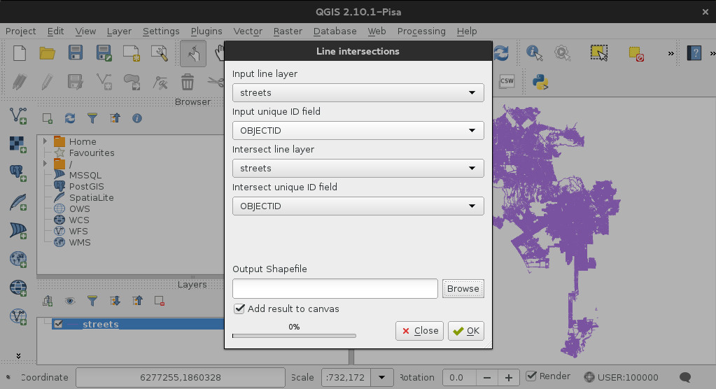
Using QGIS, we turned the circulation file, which is essentially a bunch of lines, into a bunch of intersections (points). (Menu:Vector > Analysis > Line Intersections). You want to intersect the circulation layer with itself, leaving the OBJECTID as the unique identifier.

These are pretty large data sets, so some of the operations can be really slow. To speed things up while we perfected our process, we cropped out everything except a small neighborhood within LA. Once we had our process down, we ran through it again on the entire data set.

Now, because our newly created intersections are points, we need to calculate a small buffer that represents the “area” of the intersection around each point. To simplify analysis, we assume that all collisions within 30 feet of the intersection should be considered.

We arrived at this number (30ft) empirically by comparing the number of accidents at 10, 20, 30, 40, and 50 foot buffers around the intersection. Our data showed a sharp leveling off after 30 feet.

Create a new buffer (Menu: Vector > GeoProcessing Tools > Buffer). Select your new intersections layer as the input vector layer, and set buffer distance to 30. Save your output shapefile as “intersection buffers”.

Collisions

Starting with SWITRS, which contains all collisions, we want to get just those collisions where a cyclist was injured. Add the Collisions03to12.shp as a new vector layer. Right click on the layer to open the attributes table. Filter the records in the attributes table. Filter the records where 'BICCOL' = 'Y'.

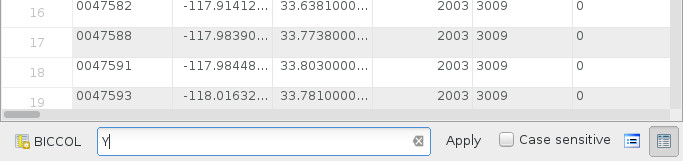
After applying the filter, our attribute table has only bicycle collisions. Select all the rows (ctrl + a or cmd + a on mac). Then press the “copy selected rows” button. Back in the main QGIS window we paste the features as new vector layer (Menu: Edit > Paste Features as > New Vector Layer). Call the new layer “bicycle collisions”.

Combining the Two

Now, we want to count all the collisions that occurred within each one of these buffers. We can do this using the QGIS Points in Polygon feature, (Menu: Vector > Analysis > Points in Polygon). Input polygon vector layer should be the intersection buffer and the Input point vector layer should be the bicycle collisions layer.

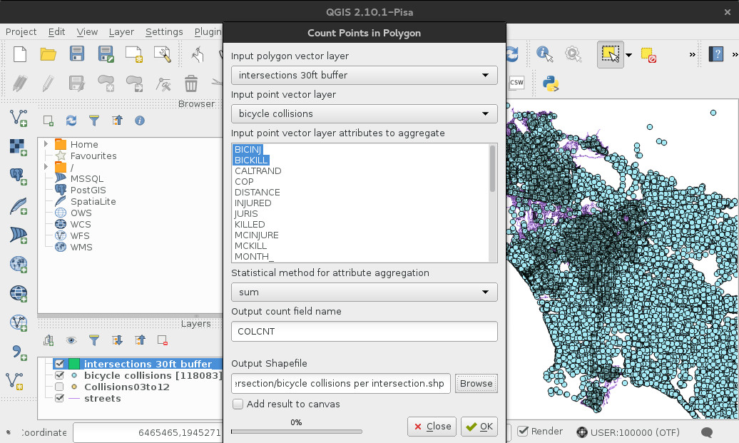
Select the BICINJ and BICKILL columns to aggregate the number of injured and killed cyclist per intersection. Make sure you’re using sum to aggregate your columns and rename the output count filed to COLCNT. Call your output shapefile “bicycle collisions per intersection” and save.

Inspect the attributes table of that new layer, sort by count, and viola. LA’s most dangerous intersections for cyclists.

If you had any questions, or comments please let us know so we can improve this article. Also, we’d love to help you get involved in doing analysis with this data yourself.